Integration is a fundamental problem in mathematics and computer science with many applications that span the whole spectrum of sciences and engineering. It appears, for example, in problems in statistics, biology, and economics, to name a few concrete application areas. Integration of functions non-rectangular domains like a general convex body or say a polytope turns our to be a difficult task to solve directly. Also, for higher dimensional integral calculation around defined integration limits can be more harder task while dealing with so many variables. To rule out this difficulty, Monte Carlo Integration is used. The overview can be found here for this algorithm.
What is Monte Carlo Integration?
In mathematics, Monte Carlo integration is a technique for numerical integration using random numbers. It is a particular Monte Carlo method that numerically computes a definite integral. While other algorithms usually evaluate the integrand at a regular grid, Monte Carlo randomly chooses points at which the integrand is evaluated.This method is particularly useful for higher-dimensional integrals. Also it can be used to integrate functions around a \(N\)-dimensional polytope. Wikipedia]
A naive example using acception-rejection sampling
Here is a way to estimate the area of the circle using Monte Carlo Integration by acception-rejection sampling.
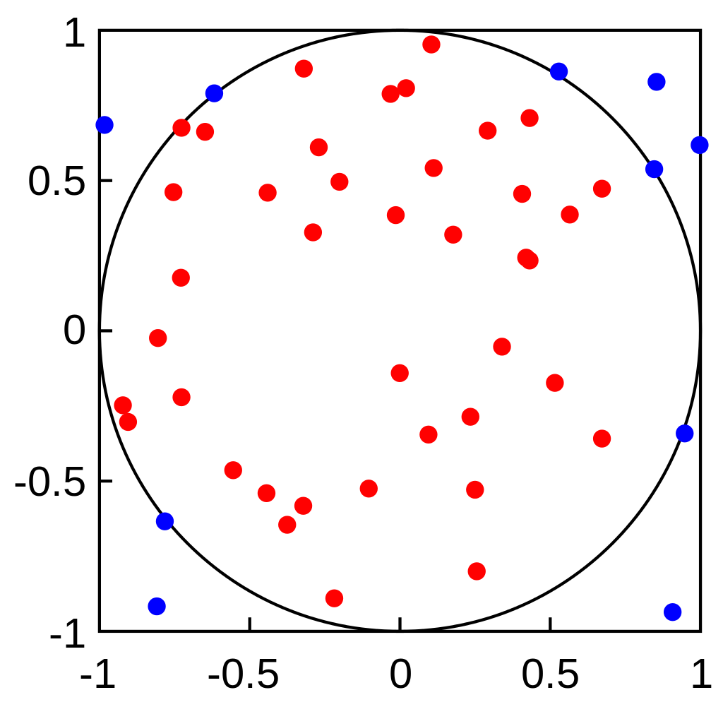
A circle around the origin of radius = 1, say \(x^{2} + y^{2} = 1\) is inscribed inside the square. We know the area of circle is \(\pi r^{2}\), but just assume we don’t know the value of \(\pi\). How are we supposed to calculate the circle’s area?
Here comes the use of Monte Carlo Integration Algorithm.
- We take randomly sample points inside the square of side \(s\) which contains our desired circle whose area we wish to calculate.
- We check if each \(2\)D random point is inside the circle or not. It is easy to check: Say we have a sampled point \((x,y)\) and we can check if \(x^{2} + y^{2} \le 1\).
- Say we check this for \(N\) sampled points inside a
forloop. Let us use a loop counterint accepted = 0. - If the point satisfied which are the red points in the image,
accepted++, for the blue points they are rejection points and and are not counted. - Now as we are supposed to know the volume of the subspace which is a square that is \(s^{2} = 4\) square units.
\(\begin{equation*} \displaystyle Area\; of \; Circle = Area \; of \; Square \cdot \dfrac{accepted}{N} \end{equation*}\)
An example using function evaluation at sample points
A little different example when we are not dealing with the acception-rejection sampling area and the entire subspace \(K\) is our integration domain and our sampling area. In here we evaluate the function at each point. Suppose we take an integration function \(f(x) = e^{-x^{2}}\). Since the function has depends on one variable only that is, \(x\), it is supposed to be 1-dimensional function and we wish to integrate it from \(-1 \le x \le 1\).
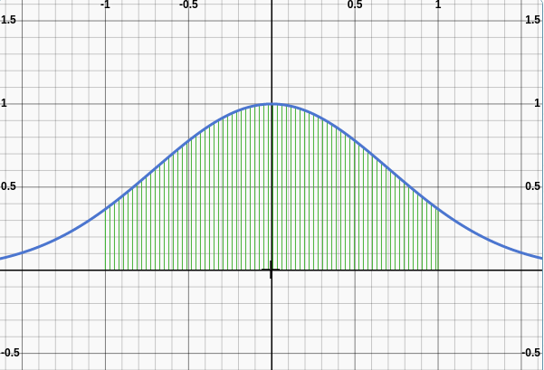
- We start off by taking random sample points inside our subspace that is \(x \in [-1,1]\).
- Suppose for \(N\) sample points we run the loop \(N\) times.
- We evaluate the function at each point and take the overall sum.
sum += F(X), where X is our sampled point. - Volume of the subspace is 2 units i.e. \(volume(K)\).
\(\begin{equation*} \displaystyle \int_{K} f(x) = volume(K) \cdot \dfrac{sum}{N} \end{equation*}\)
Similar Software
The Project: Simple-MC-Integration
To make it easy and more understandable let us break it into some easy terms.
- Subspace K : The integration domain around which the function is meant to be integrated. The points which are sampled are taken from this subspace as well. This subspace is a polytope, a convex \(n\)-dimensional body, where \(n > 0\).
- Integration Function : The integration function is also supposed to be the same dimensions as the convex body K. Let the function be \(f(x_{1},x_{2},...,x_{n})\) or just by \(f(X)\). [Here, \(X\) represents a \(n\)-dimensional cartesian point in \(n\)-dimensional space i.e \((x_{1},x_{2},...,x_{n})\)].
- Sampling : The sampling as above mentioned in the examples it will not be done here by taking random points. To ensure uniformity of the sampled points inside the polytope, random walks is supposed to be use here to ensure greater accuracy and efficiency. It is feature from volesti library in random walks directory by volume approximation by GeomScale.
Types of random walks offered here for sampling are BallWalk, BilliardWalk, AcceleratedBilliardWalk, JohnWalk, DikinWalk, VaidyaWalk and RDHRWalk.
The integration domain which is a polytope (\(n\)-dimensional convex body) in H-representation. Polytopes can be represented using H-representation to store cubes, rectangles, simplices, product simplices, cross-polytopes, birkhoff polytopes. Such polytopes are can be created using Volesti libraries itself, represented in the form \(AX \le b\), where \(A\) | \(b\) is family of hyperplanes of in the form mentioned below.
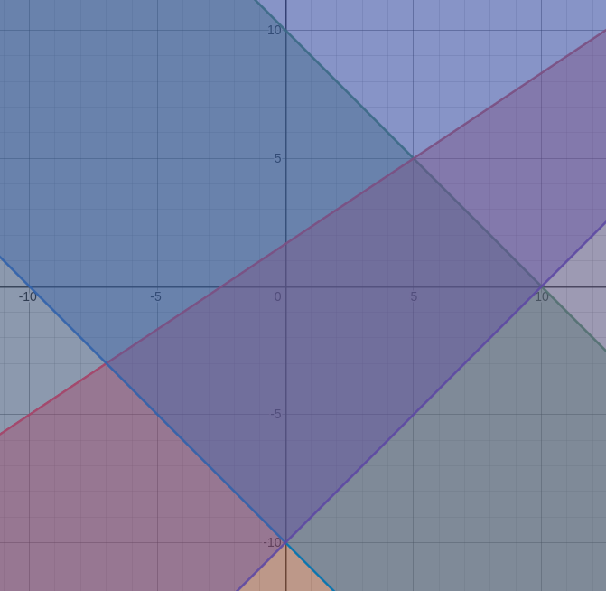
Suppose a polytope is defined in H-representation(using a family of hyperplanes and forming a closed convex figure). For example we take a quadrilateral bounded by 2D linear equations and the closed quadrilateral is satisfied by the following constaints:
\(x_{1} + x_{2} \le 10\)
\(-2x_{1} + 3x_{2} \le 5\)
\(-x_{1} - x_{2} \le 10\)
\(x_{1} - x_{2} \le 10\)
They can be represented in the form of \(AX \le b\), where
\(\begin{equation*} A = \begin{bmatrix} 1 & 1 \\ -2 & 3 \\ -1 & -1 \\ 1 & -1 \end{bmatrix} \end{equation*}\) \(\begin{equation*} \qquad X = \begin{bmatrix} x \\ y \\ \end{bmatrix} \end{equation*}\) \(\begin{equation*} \qquad b = \begin{bmatrix} 10 \\ 5 \\ 10 \\ 10 \end{bmatrix} \end{equation*}\)
\(A\) is a \(4 * 2\) matrix, \(X\) is \(2 * 1\) matrix and \(b\) is a \(4 * 1\) matrix. For more detailed insight about convex sets, you can study them from here.
If the user prefers to enter integration limits in the \(n\)-dimensional space, there is a provision for the same too. You can jump to usage section on this page to study more about it.
For volume calculation, there are three algorithms in the Volesti library that is, SOB(Sequence of Balls), CG(Cooling Gaussians) and CB(Cooling Balls).
As mentioned above, we are going to calculate the integral pretty much in the same way rather use some professionalism using random walks and volume algorithms.
- We start by taking random sample points inside our our subspace \(K\).
- Suppose for \(N\) sample points we run the loop \(N\) times.
- We evaluate the function at each point and take the overall sum.
sum += F(X)\(\) is our sampled point. - Volume of the convex body i.e. a polytope, let it be \(volume(K)\).
\(\begin{equation*} \displaystyle \int_{K} f(x) = volume(K) \cdot \dfrac{sum}{N} \end{equation*}\)
simple_MC_integration.hpp contains the header file written for the above algorithm mentioned. [Link]
Simple-MC-Integration is the first part of my Google Summer of Code 2021 project. The second part is the Lovasz-Vempala Monte Carlo Integration. You can jump to that blog here!
Testing
Integral values have been tested using latte integrale, state of the art software for polytope volume calculation and integral calculator for functions around surrounded by a polytope. The remaining details are equipped in the README.md itself. [Link to the Latte Tests]
simple_mc_integration.cpp contains the tests written. [Link]
Usage
Here is a miniature code to show the use the simple_mc_integration.hpp functions. There are two of them.
Some prerequisite information:
NTis defined fordoubleeverywhere in the below examples.- Assume that we have already created our functions for integration. They look like this below and they are supposed to be integrated around the convex bodies i.e. polytopes or the integration limits we can define.
    // NT is double

    NT rooted_squaresum(Point X) {
	    return sqrt(X.squared_length());
    }

    NT exp_normsq(Point X) {
	    return exp(-X.squared_length()) ;
    }
- volume_approximation has features of generating polytopes by from generator function in known_polytope_generators.h You can use it to create polytopes mostly in the form of \([-1,1]^{n}\).
1. Simple MC Integrate :
- Integration limits can be defined by upper limits and lower limits. By default, limits are taken to be \([-1,1]^{n}\).
Functor Fxis the integration function.dim&Nare dimensions and number of sample points in unsigned integer format.voltypeisenumfor volume options like SOB, CB and CG. (Mentioned above)LowLimitandUpLimitrepresentsstd::vectormasked asLimitsand you can check their declaration below in the usage.walk_lengthof typeintis the length of the walk during making the random walks and taking sample points.erepresents the tolerable limits of error.- The function defined here is
simple_mc_integrate()and is stuctured as follows in C++.
template
<
    typename WalkType = BallWalk,
    typename RNG = RandomNumberGenerator,
    typename NT = NT,
    typename Functor
>
NT simple_mc_integrate (Functor Fx,
                        Uint dim,
                        Uint N = 10000,
                        volumetype voltype = SOB,
                        Limit LowLimit = lt,
                        Limit UpLimit = lt,
                        int walk_length = 10,
                        NT e = 0.1)
{
    // code goes here
}
Example code:
Limit LL{-1, -1}; // Lower limits of integration
Limit UL{1, 1}; // Upper limits of integration

integration_value = simple_mc_integrate <AcceleratedBilliardWalk> (rooted_squaresum, 2, 100000, SOB, LL, UL);
std::cout << "Example 1 integral value = " << integration_value << endl;

// default integration limits are taken to `[-1,1]^n`
integration_value = simple_mc_integrate <BilliardWalk> (exp_normsq, 5, 100000, SOB);
std::cout << "Example 2 integral value = " << integration_value << endl;
Output code:
Example 1 integral value = 3.0607
Example 2 integral value = 7.48
2. Simple MC Polytope Integrate :
- Integration limits here taken as the boundary of the polytopes.
Functor Fxis the integration functionPolytope &Pshould is passed as a reference which creates the bounds for integration and the function is supposed to be integrated around it.Nis number of sample points in unsigned integer format.voltypeisenumfor volume options like SOB, CB and CG. (Mentioned above)walk_lengthof typeintis the length of walk during making the random walks and taking sample points.erepresents the tolerable limits of error.- The function defined here is
simple_mc_polytope_integrate()and is stuctured as follows in C++.
template
<
    typename WalkType = BallWalk,
    typename Polytope = HPOLYTOPE,
    typename RNG = RandomNumberGenerator,
    typename NT = NT,
    typename Functor
>
NT simple_mc_polytope_integrate(Functor Fx,
                                Polytope &P,
                                Uint N = 10000,
                                volumetype voltype = SOB,
                                int walk_length = 1,
                                NT e = 0.1,
                                Point Origin = pt)
{
    // code goes here
}
Example code:
HP = generate_cube <HPOLYTOPE> (10, false);
integration_value = simple_mc_polytope_integrate <BilliardWalk, HPOLYTOPE> (exp_normsq<double>, HP, 100000, SOB);
std::cout << "Example 1 integral value = " << integration_value << endl;

HP = generate_birkhoff <HPOLYTOPE> (4);
integration_value = simple_mc_polytope_integrate <BilliardWalk, HPOLYTOPE> (one_sqsum, HP, 100000, SOB);
std::cout << "Example 2 integral value = " << integration_value << endl;
Output code:
Example 1 integral value = 55.20
Example 2 integral value = 0.000163